The polls, and the forecasters using them, performed pretty well. Harry Enten posted for the Guardian this morning about the overall success of pollsters in the 2012 cycle, and John Sides put up this great post/figure over at The Monkey Cage. (The figure was also picked up by Ezra Klein.)

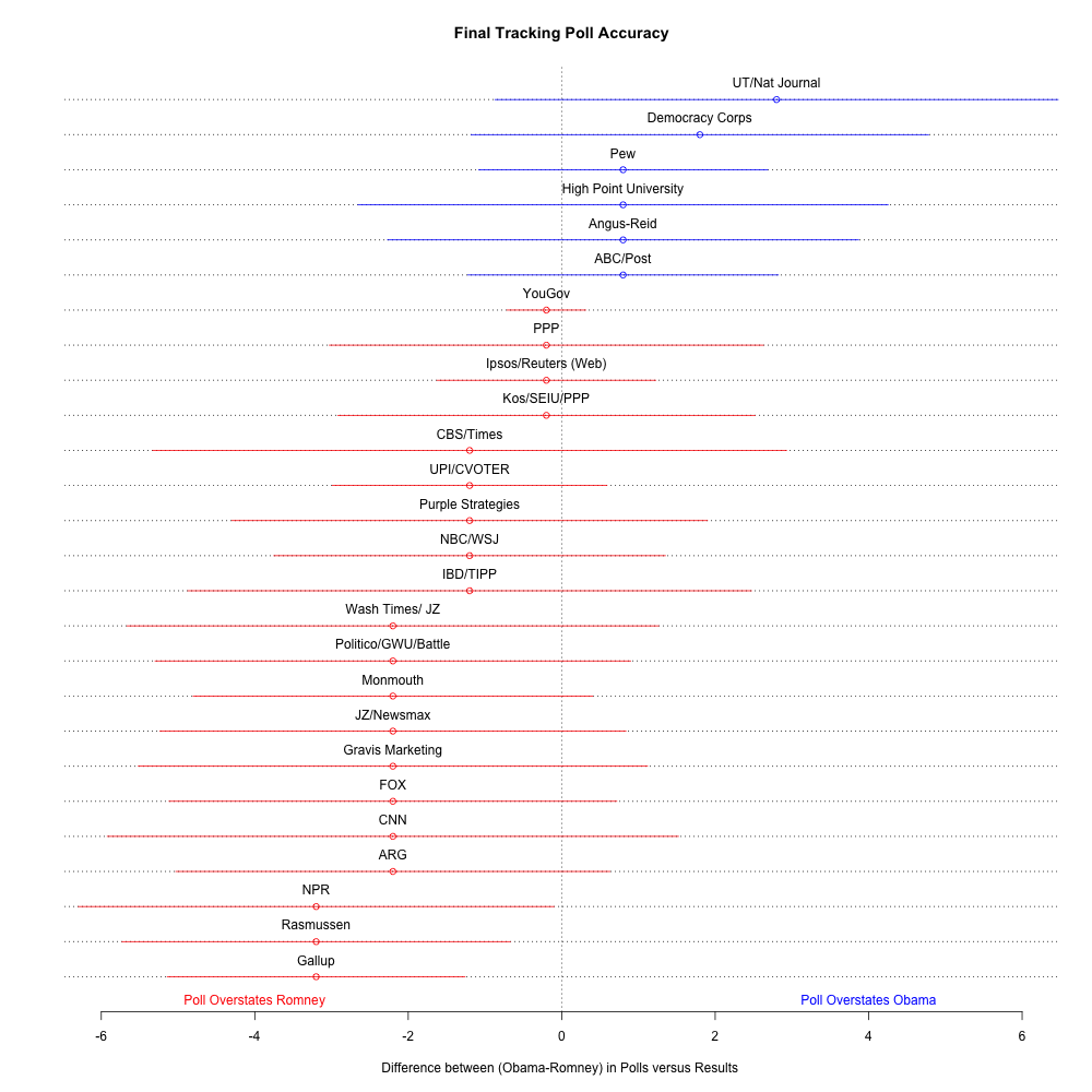
I wanted to see the estimated error margins around the final pollster predictions. So here’s my take with 95 percent confidence bands:

The figure shows the difference in the predicted and actual Obama margin. Positive numbers mean that the pollster overstated Mr. Obama’s margin of victory; the negative implies the inverse.

Almost all of the polls came within a reasonable distance from the outcome. In fact, most contained the true outcome in their margins of error.

We’re not live-blogging the presidential race, but here is an interesting tidbit:

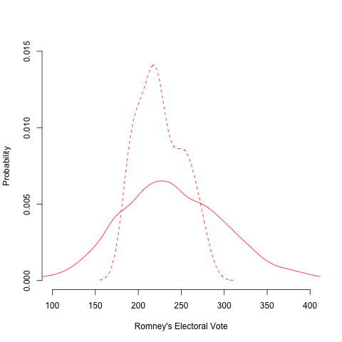
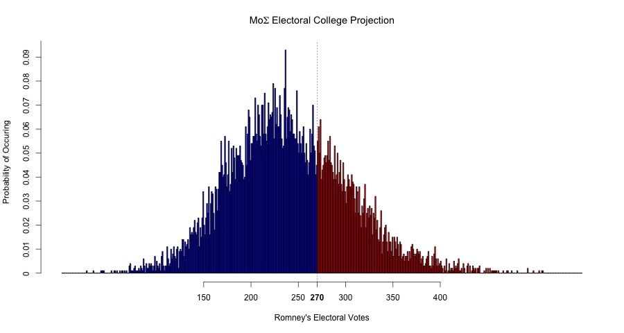
There is not much to update in the model, but we can update our expectations given current returns. Put another way: we can ditch simulations with results we know to be incorrect.

By updating our beliefs, Mr. Romney’s chances of winning drop from 32 percent to only 12 percent. As you can see in the figure, Mr. Romney’s distribution of electoral votes has become much more certain (as we would expect), but he’s lost most area under the curve to the right of 270.

The door on Mr. Romney’s probability of winning is closing, and quickly.

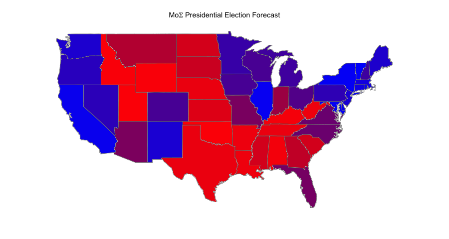
As we published yesterday, the Margin of Error forecast predicts Mr. Obama to secure reelection with 303 electoral votes to Mr. Romney’s 235. This translates roughly into a 68 percent chance for Mr. Obama to win, leaving a nonnegligible 32 percent chance of an upset victory by Mr. Romney.

One of the more interesting elements of the model is that it’s agnostic to state-level polling. Most of the highly-trafficked forecasting models (the gold standard is Nate Silver’s 538 model) use various methodologies for aggregating state- and national-level polling.

The MoE forecast, on the other hand, uses very few variables. The national popular vote is predicted using late-season approval data; the state-level votes are forecast using (a) previous election results; (b) August-November change in unemployment; (c) home state advantage; and (d) a regional dummy variable. No polls.

Despite the stark difference in methodology, the forecast comes in well in-line with most quantitative models. The most notable gap between our model and many of the poll-aggregation models is, in fact, that ours makes a far more conservative prediction of uncertainty.

So, what’s the deal with this fundamentals-based model, anyway? In my opinion, a fundamentals-based forecast brings some distinct advantages and disadvantages.  Continue reading →

Over the summer, we published a forecast for the 2012 presidential election based solely on election-year fundamentals. On the evening before Election Day, I am republishing the forecast. The only changes since summer come in the form of updated economic variables and approval numbers.

The model predicts Mr. Obama to win 51.5 percent of the national two-party vote to Mr. Romney’s 48.5 percent. Propagating these predictions to state-level results, the model forecasts Mr. Obama to secure 303 electoral votes to Mr. Romney’s 235.

Over 10,000 simulations, Mr. Obama wins the election 68 percent of the time.

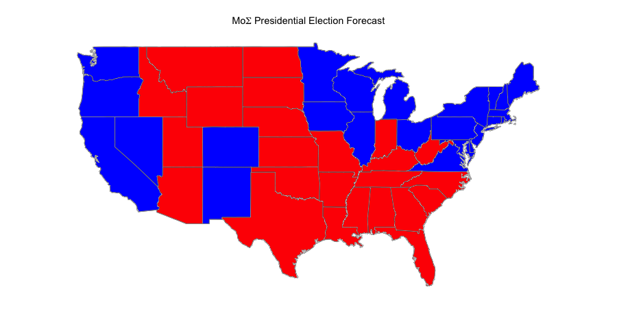
The model rests pretty comfortably in line with other social scientific models.

As I will expand on in a later post, one of the notable elements of the model is that it does not account for horserace polls. Unlike the models that get the most attention, this one only incorporates economic fundamentals for state-level predictions.

Accordingly, the model likely understates Mr. Obama’s advantage in Ohio, where the auto bailout seems to have made a dent in Mr. Romney’s chances. Working in the opposite direction, the model seems to overestimate Mr. Obama’s chances of winning Colorado, which most forecasts predict to be exceptionally close while the model gives Mr. Obama 53 percent of the two-party vote. For Colorado in particular, the model seems to be overly reliant on Mr. Obama’s favorable result there in 2008 and the state’s decent unemployment trajectory.

On the flip side, the model does not suffer from what’s undoubtedly haunting many Democrats: the chances that polls, with low response rates and undersampled cell-only households, are systematically incorrect. Put simply: without polling data included, the model doesn’t require polls to be accurate.

The model still comes with considerable uncertainty. In fact, the model may be  overly cautious. Nate Silver’s model, for example, gives Mr. Obama a roughly 20-percent higher probability of winning than ours. That stems from multiple levels of uncertainty that we’ve added to the model: at the national, regional, subregional and state levels.

Though we can coerce the model into predicting a binary outcome in each state, we must note that several states are really too close to make a meaningful prediction. In particular, Virginia, North Carolina and Florida are forecast to come within a razor-thin margin of 1 point or less. Those states are, according to this naïve model, way too close to call.

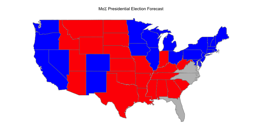
All told, the model holds pretty closely to what we are seeing from other prominent models. Mr. Obama holds a definitive lead going into Election Day. Indeed, even were all too-close-to-call states to fall into Mr. Romney’s column, Mr. Obama would still secure reelection.