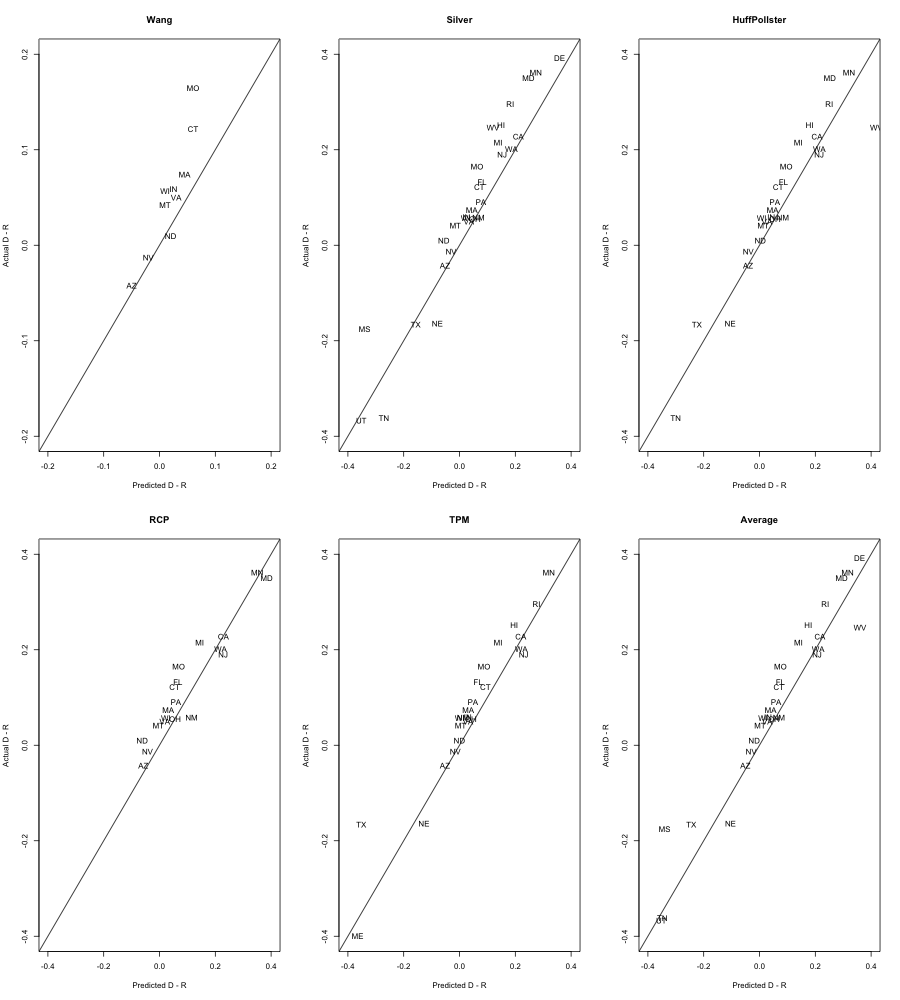
Last week, we examined the accuracy of several presidential forecasts. For those familiar with statistics and probability theory, the results proved unsurprising: the forecasts came reasonably close to the state-level outcomes, but the average forecast outperformed them all.

Put another way, the aggregate of aggregates performed better than the sum of its parts.

This year’s Senate races provide us another opportunity to test our theory. Today, I gathered the Senate forecasts from several prognosticators and compared them to the most recent Election Day returns. As before, I also computed the RMSE (root mean squared error) to capture how accurate each forecaster was on average.

We must note one modest complication: not all forecasters posited a point-estimate for every Senate race. Nate Silver put forward a prediction for every race; but Sam Wang of Princeton University only released 10 predictions for competitive races.

We accordingly compute two different RMSEs. The first, RMSE-Tossups, only computes the RMSE for those races for which each forecaster put forward a prediction. (There are nine races that fall into this category: Arizona, Connecticut, Massachusetts, Missouri, Montana, Nevada, North Dakota, Virginia and Wisconsin.)

The other calculation, RMSE-Total, shows each forecaster’s RMSE over all predictions. Wang, for example, is evaluated by his accuracy on the ten predictions he made; while Silver is evaluated on all 33 races.

Forecast	RMSE-Tossups	RMSE-Total
Wang	4.7	4.6
Silver	5.1	8.0
Pollster	3.8	5.8
RealClearPolitics	5.4	5.1
TalkingPointsMemo	3.9	8.0
Average Forecast	4.4	5.4

The numbers in the above table give us a sense of how accurate each forecast was. The bigger the number, the larger the error. So what can we learn?

Alas! The average performs admirably yet again. It’s not perfect, of course; for some races, there are precious few forecasts to average over: Delaware, for instance, has only the 538 prediction.

To begin accounting for this, we weight the RMSE by the share of forecasts used to compute the average. If we limit our evaluation of the average to only those races with three or more available forecasts, the RMSE drops to 4.8.

What else emerges from the table? For one, the poll-only forecasts — especially the Wang, RCP and Pollster forecasts — perform better than Nate’s  mélange of state polls and economic fundamentals.

North Dakota, where Democrat Heidi Heitkamp bested Republican Rick Berg, provides a case in point. Pollster and RealClearPolitics both predicted a narrow win for Ms. Heitkamp. The 538 model considered the same polls upon which Pollster and RCP based their predictions; but the fundamentals in Mr. Silver’s model overwhelmed the polls. As a result, the 538 model predicted that Mr. Berg would win by more than five points. [See Footnote 1.]

 

In sum, however, all of the forecasts did reasonably well at calling the overall outcome. We can chalk this up to another victory for (most) pollsters and the quants who crunch the data.

1. Addendum: In the original post (text above is unchanged), I argued that Mr. Silver’s economic fundamentals pushed his ND forecast in the wrong direction. This undoubtedly contributed to his inaccuracy in North Dakota, but it wasn’t the main factor. As commenters pointed out, Silver’s model was selective in the polls it used to predict the outcome. As of the last run of the model, Silver’s polling average lined up fairly well with RCP (Berg +5) but not with Pollster (Heitcamp +0.3). Mea Culpa.