
Last week, a friend asked for my opinion on an economics problem where students were asked to estimate the statistical value of a human life.

This will make more sense later…
The procedure blew my mind, and not in a good way. Not because I’m not a fan of quantifying the value of life — it’s weird, but I’d rather governments use good estimates over bad ones — but because the statistics are being used so poorly.
And it wasn’t my friend’s fault. He was following the example of several scholars who used the same framework to answer this question. And he got the problem set question correct, despite it being horrifyingly misguided.
Regression to the Rescue!
Here’s the published article by James Hammitt with the economic theory, here’s an overview of the field by Viscusi & Aldy (2003), and here are some applications. Basically, we’re trying to pin down how much you would spend to reduce your risk of death by some fixed amount. So, for example, how much is it worth to you if I could reduce your chance of death this year by, say, 0.1 percent?
Unfortunately it’s expensive and theoretically questionable to ask people that question. Even if we could afford the survey, do we think people could respond to the hypothetical accurately? I couldn’t.
So we flip the task toward figuring out how much we demand to be paid to undertake dangerous jobs. And since we’re in econometrics land, let’s start with linear regression. With some controls (age, blue collar, race, et cetera), let’s find the relationship between the dangerousness of a job (risk of death) and compensation (weekly wages). Economists call this a hedonic wage model.
And then? Let’s predict wages where risk of death is certain, i.e., p = 1.0. Or, as Moore & Viscusi (1986) put it, “We extrapolate the willingness to pay of the individual worker for a small risk reduction linearly to calculate the collective willingness to pay for a statistical life.”
Voilà! Now we know how much people value their lives.
See the problems yet?
When my friend first showed me this approach, I laughed a bit. His response went something like this:
Yea, I know, it’s not great. We only have a sample of 300. And we don’t have all of the variables we would want, so there may be some omitted variable bias, right? So it’s not perfect, but…
He’s right. Fitting a linear model without including relevant variables results in biased estimates. Proving this is simple but isn’t really where my objections lie.
My problem comes from the ridiculous extrapolation involved here. Let’s assume that we have the relevant variables in hand. Even under this unlikely condition, extrapolating so far beyond the data can make us super confident in an utterly stupid model and its predictions.
A simulated example
To show what I mean, we will use some simulated data. By using data that we create ourselves, we can observe the “truth” in a purely objective way, and thus test our intuition about lots of stuff. For the following demonstration, I’ll give the basic overview and give technical details after the post.
Let’s assume that we have some variable  that represents “risk of death” in various occupations. Now let’s assume that nature defines some true function linking “risk of death” to wages, and the function is arbitrarily complicated:
}{1-x_i} + \epsilon_i")
There’s nothing special about the function, other than that I (acting as ‘nature’) defined it myself. It also has a nice asymptote at  1, meaning that the limit from the left
  = \infty") . This comes from the denominator (since dividing by 0 is undefined), and could match some intuition about nobody accepting any reasonable wage for a risk
. This comes from the denominator (since dividing by 0 is undefined), and could match some intuition about nobody accepting any reasonable wage for a risk  1. The error term
  we will assume to be normally distributed with expectation of zero.
With this function in hand, we can randomly generate some values for x that could reasonably be risks of death; in this case, for ease, ") , meaning uniformly distributed on the interval 0 (risk=0%) to 1 (risk=100%).
, meaning uniformly distributed on the interval 0 (risk=0%) to 1 (risk=100%).
If we fit the linear model to the full data (because this data is costless, let’s say n=10,000), we’d see pretty quickly that regressing y on x is a terrible idea. The estimated coefficient on risk of death is significant (with 10,000 observations it’s hard not to get ‘significant’ coefficients; see here and here); but the plot of predicted values  against y make it pretty obvious that the model misses the mark:
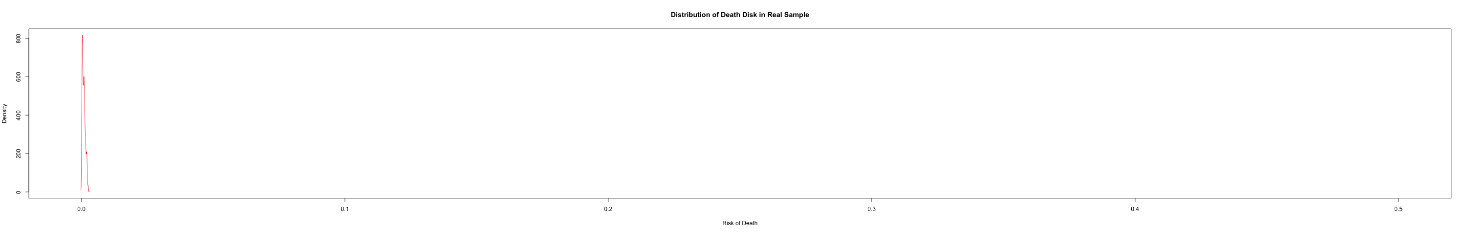
Here’s the problem: we don’t have the full data. Nobody accepts jobs where the risk of death  , or really anywhere near it. The highest occupational risks seem to have ~120 deaths per 100,000 workers. The data my friend was given for his homework, similarly, had the following risk density (and for amusement, see here for perspective):
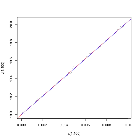
So, for verisimilitude, let’s refit the model using only a small subset of the data from the low-end values of x, say those for which 0<x<0.01. Now things get frighteningly fun…
Again, the coefficient estimate is significant, but this time there’s nothing in the residuals that give us pause:
In fact, there’s nothing to point out exactly how wrong our model is! For example, check out this image which shows the “true” line and the linear fit line. You can’t distinguish one from the other. In this restricted sample, the root mean squared differences between the linear fit and the true model is only 0.002, compared to more than 13,000 between the true versus linear fit values in the full data.
How bad could this possibly be? Well, let’s plot the true function in black and the linear fit in grey:
Oh, right. We could be really, really far off. Oops.
That was a fun exercise, but so what?
Why does any of this matter? First, consider this fact: I provided us with one possible true function, just for comparison with our linear model. But the actual relationship between risk and wages, to the extent that we can say it exists at all, could take any form.
Second, and this is the scarier part, it’s entirely possible to fit a linear model that looks perfectly acceptable. Within the small subset of data, the linear model is a decent approximation of the truth, at least insofar as we might be interested in predicting wages from risk.
In extrapolating so far beyond the data, however, we assume that this decent approximation works for all values of x, even with no evidence to support the assumption. There’s no data out at the extremes to tell us how good or bad the assumption is, and thus not only is our model likely wrong, but there is effectively no bound on how wrong we might be.
This isn’t too different from me telling you that the relationship between, say, age and income, can be approximated by a linear model. We’ll include a squared term since income at upper ages tends to fall below our full earning potential. And then - because the model fits so well for data we have! - I’ll extrapolate to give you the expected income for somebody who is 200 years old (it’s less than negative $500,000… someone should stop researchers from improving life expectancy, stat!).
E(income | age=200) ~ <-$500,000… or something. Scale on the y-axis is categorical from 0 ($0) to 16 ($500,000+). The rug plot at the bottom shows the range of actual data in the CCES. Everything else is just a really bad guess.
Third, no standard ‘fix’ in the econometric toolkit is going to help us. Unlike our toy data, we aren’t ignoring data that might exist out there somewhere. We’re extrapolating beyond data that will likely ever exist. On our subsample, even transforming x with the true function - the function that we’d never know was correct a priori - gives us predictions indistinguishable from the linear fit.
In short, we will never know how wrong we are, in which direction, or how to improve the model.
So what do you propose?
When I pointed out the extrapolation issue to my friend, he responded with some frustration: “We need an estimate, and this is as good a method as any. What do you want governments to do? Guess?”
Well, yea, kinda. I would rather a government or agency guess, and be transparent about it, than use the prediction from a hedonic wage model. The linear extrapolation is just a poorly founded guess anyway, since the method was not designed nor is it suited to the question at hand. Masking it as some scientific method for defining a quantity of interest gives it an air of authority that it doesn’t deserve.
To put it another way, I can buy a car to get us from New York to London. But hey, at least I bought a vehicle of some variety, right? Except that we’ll both drown, and you’ll wish you hadn’t trusted my whole “look, it’s a fancy machine” argument.
Now, I don’t have a better alternative at the moment. Asking people seems silly, and besides, that could also result in dumb linear modeling. Guessing isn’t satisfactory. So what to do?
Well first, please stop defining everything as a regression problem. As a wise man should never have had to write (but did): “Linear regression is not the philosopher’s stone.” Let’s stop treating it like one.
And second… wait, I’ve written 1,500 words and - if you’re still with me - I owe it to the reader to stop. Also, I don’t have an answer right now. I leave that open to intrepid readers. E-mail or comment, and maybe there’s a follow-up post in the near future.